


Forecasting Inflation Data Using EViews: A Step-by-Step Guide
Forecasting Inflation Data Using EViews: A Step-by-Step Guide

Are you looking for a comprehensive guide on forecasting inflation data using EViews? Look no further! In this step-by-step guide, we will walk you through the process of predicting inflation rates using EViews, a powerful statistical software. Whether you're a beginner or an experienced analyst, this article will provide you with the necessary knowledge and insights to confidently forecast inflation data and make informed decisions. From collecting and organizing data to selecting the appropriate models and interpreting the results, we've got you covered. Join us on this exciting journey as we dive into the world of inflation forecasting with EViews. Get ready to unlock the secrets behind accurate predictions and take your data analysis skills to the next level.
We will provide you with a comprehensive overview of how to forecast inflation data using EViews.

Data Acquisition and Setting the Sample Period
Data Source: We begin by obtaining the inflation data(CPI) from the Federal Reserve Economic Data (FRED). Our dataset spans from January 1948 (1948m01) to November 2023 (2023m11).
Defining the Sample Period in EViews: For our analysis, we set the focus of our study to the period from January 1948 (1948m01) to September 2023 (2023m09). This is done to ensure that our analysis is based on complete data and avoids the inclusion of partial or forecasted figures for the remaining months of 2023.
Creating the ARMA Model Equation
Understanding the Equation: We will analyze the inflation data using an ARMA model, specifically an AR(1) MA(1) model. This means our model will include one autoregressive term (AR(1)) and one moving average term (MA(1)). The AR term captures the momentum and direction from previous values, while the MA term adjusts for past errors in the predictions.
Equation Setup in EViews: In EViews, we construct the equation for our model as
inflation c AR(1) MA(1). Here, 'inflation' represents our variable of interest, 'c' stands for the constant term in our equation, 'AR(1)' adds the autoregressive component, and 'MA(1)' incorporates the moving average component.
Analysing of the Equation
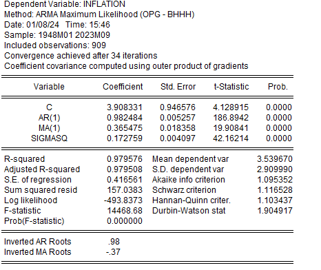
Model Specification: The model is an ARMA(1,1), which means it includes one autoregressive term (AR(1)) and one moving average term (MA(1)). This model is appropriate for time-series data where current values are influenced by both their past values and past forecast errors.
Coefficients:
The AR(1) coefficient is close to 1 (0.982), indicating a strong persistence of inflation over time. This means current inflation is heavily influenced by the inflation of the previous period.
The MA(1) coefficient is about 0.365, which shows the extent to which the previous period's forecast error affects current inflation.
Statistical Significance: All variables, including the constant term, AR(1), and MA(1), are statistically significant with p-values of 0.0000, as indicated in the 'Prob.' column.
Model Fit:
The R-squared value is 0.979, and the adjusted R-squared is 0.979, which are both very high. This suggests that the model explains a large proportion of the variability in inflation.
The F-statistic is significant, indicating the overall significance of the regression model.
The Durbin-Watson statistic is approximately 1.90, which is close to the value of 2, suggesting that there is no major issue with autocorrelation of residuals.
Diagnostics:
The Inverted AR Roots and MA Roots fall inside the unit circle (since they are less than 1 in absolute value), which suggests that the model is stable and the processes are stationary.
The results suggest that the model is well-specified and provides a good fit to the historical inflation data. This model can be a useful tool for understanding the behavior of inflation and for making short-term forecasts.
Dynamic Forecasting
We need to click the forecast button in equation screen.

We are preparing to run a dynamic forecast in EViews for the inflation series. Here's a step-by-step explanation of how to proceed with this:
Selecting the Forecast Type: In the forecast dialogue box, we have selected 'Dynamic forecast'. This method will use the estimated coefficients from your ARMA model to generate forecasts that incorporate information from previous forecast errors. This means the forecast for each period will use the forecasted value from the previous period as part of the input.
Setting the Forecast Sample: We have specified the forecast sample to be from September 2023 to November 2023 (2023m09 2023m11). This indicates we are looking to predict the inflation values for a two-month period using the model.
Naming the Forecast: We are prompted to give a name to our forecast series: 'inflationf_od'. This will help we identify the forecasted data in our EViews workfile.
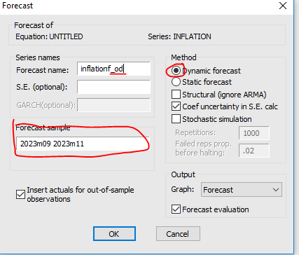

Once you click 'OK', EViews will generate the dynamic forecast based on your ARMA(1,1) model.

Performance Metrics:
Root Mean Squared Error (RMSE): The RMSE is 0.5177, which measures the average magnitude of the forecast errors. It's a key indicator of forecast accuracy; the lower the RMSE, the better the forecast.
Mean Absolute Error (MAE): The MAE is 0.454, another measure of forecast accuracy, representing the average absolute errors.
Theil's U2 Coefficient: A value of 0.072 indicates a good forecast quality, as values closer to 0 suggest better accuracy.
Graphical Representation:
The blue line represents the forecasted inflation rates.
The green line indicates actual historical inflation rates.
The orange dotted lines show the confidence interval, calculated as two standard errors above and below the forecast.
The metrics suggest the model has performed reasonably well, with relatively low error measures. The graph visually confirms that the forecasted values are close to the actuals, within the confidence intervals. This model can be a useful tool for policymakers, economists, and analysts interested in inflation trends.

Static Forecasting
In this step, we are preparing to run a static forecast for the inflation series using EViews. We choose 'Static forecast' as the method, which implies that we use the model's estimated coefficients to forecast future values, assuming that the past observed values (up to the end of the estimation sample) are the only available data, and future values are not informed by any subsequent forecast errors.
We have named our forecast series 'inflationf_os' to differentiate it from other forecasts we may have conducted. This label will help us track and compare different forecast iterations within EViews.
Next, we specify the forecast sample from September 2023 to November 2023 (2023m09 2023m11). This range delineates the time period for which we want to generate forecast values.

After setting the parameters, we would proceed by clicking 'OK' to generate the forecast. Once you click 'OK', EViews will generate the static forecast based on your ARMA(1,1) model.

The Root Mean Squared Error (RMSE) is 0.253, a measure indicating the standard deviation of the prediction errors. A lower RMSE reflects a more accurate forecast.
The Mean Absolute Error (MAE) is approximately 0.189, which provides an average of the absolute errors between the forecasted and actual values. This metric is useful because it gives a direct interpretation of error magnitude on average.
The Theil U2 Coefficient is about 0.896, which is a relative measure of forecast accuracy compared to a naïve model. A value less than 1 indicates that the forecast is better than the naïve benchmark.
In the graph, the forecasted inflation values are depicted by the blue line, while the actual historical inflation values are shown with the green line. The orange dotted lines represent the forecast's confidence interval, which is plus or minus two standard errors from the forecasted value.
The metrics and the graph together suggest that the static forecast has performed well, with errors that are relatively low and within an acceptable range. The forecast seems to provide a reliable projection of inflation trends for the specified period.

Forecasting 2023 December Inflation
We understand that the static forecasting is more accurate than the dynamic forecasting and we decide to forecast 2023 December inflation with the static forecasting method.
Adjusting the Sample Range: To forecast for just 1 month, we need to ensure our sample range for estimation ends one month prior to the period we want to forecast.

The screenshot shows the series object named "inflation" within EViews, displaying monthly data points with an NA (not available) for December 2023. This indicates that we have actual inflation data up to November 2023, and we are looking to forecast the missing value for December 2023.

Here are the steps we will follow to generate the forecast for December 2023:
Open the Equation: We will navigate to the equation that contains our ARMA model used for forecasting inflation.
Set the Sample: We will ensure the sample used for the estimation ends in November 2023, the last period for which we have actual data.

Specify Forecast Details:
In the 'Forecast' window, we will input the name for our forecast series, for instance, "inflationf_1m" to signify a 1-month forecast.
We will set the 'Forecast sample' to 2023M12, which is the single month we want to forecast.
Execute the Forecast: With the forecast parameters set, we will execute the forecast. EViews will use the ARMA model to predict the value of inflation for December 2023.

Dont remember that November 2023 was %3.12.
Our result for December 2023 is %3.15.


Engin YILMAZ (
)